Autoencoders

What are autoencoders?

An autoencoder is a neural network that reconstructs a high dimensional input through a compressed lower dimension bottleneck.

The idea for autoencoders is to take a high dimensional input, compress it to a lower dimension that represents the image’s features, and then reconstruct the image from the bottleneck. The autoencoder is essentially like a dimensionality reduction method like PCA (Principal Component Analysis)

The idea was originally from the 1980s and was later promoted by Hinton & Salakhutdinov, 2006[1]

Structure of Autoencoders

The autoencoder consists of two section:

• The encoder - Takes the high dimensional input and compresses it to a latent low dimensional code which is a vector.
• The decoder - Tries to reconstruct the original input given the bottleneck.

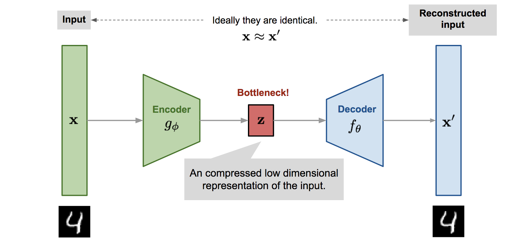
Explanation

The model has the encoder function $g(.)$ which parameterized by $\phi$ and the decoder function $f(.)$ parameterized by $\theta$. The latent code $\mathbf{z} = f_\theta(.)$. Therefore, the reconstructed input is a function $\mathbf{x'} = f_\theta(g_\phi(.))$. The aim is for the model to reconstruct the input such that $\mathbf{x'}\approx\mathbf{x^{(i)} }$ These parameters are learnt together by the model to get the output. Now, to quantify the output of the model a simple loss MSE is used

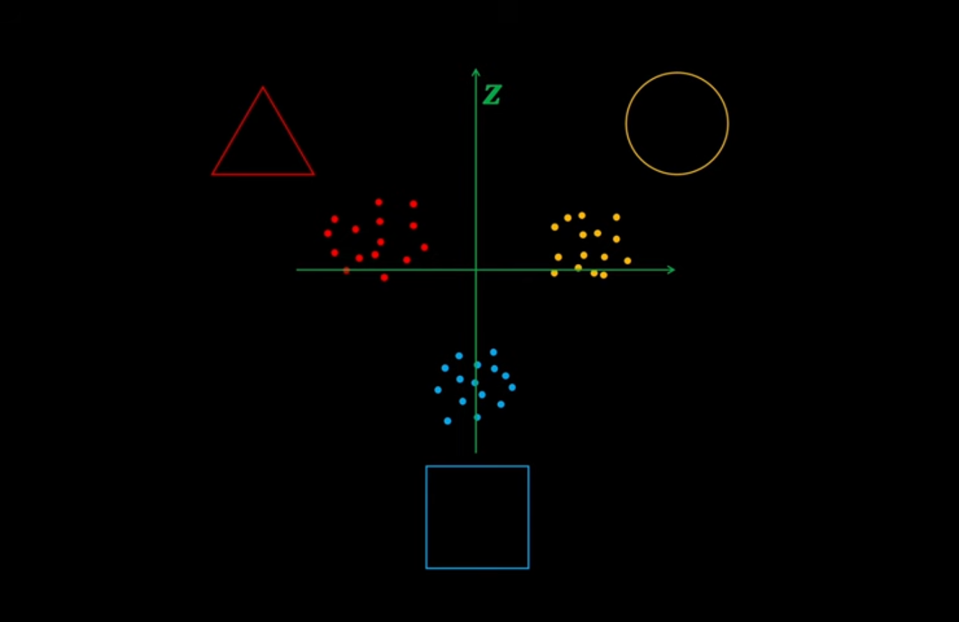
$$ Loss(\phi, \theta) = \frac{1}{n} (\mathbf{x^{(i)}} - \mathbf{x'})^2 $$

---

Lets take an example of a dataset $D$ with datapoints {$\mathbf{x^{1}}, \mathbf{x^{2}}, ... \mathbf{x^{i}}$} with mammals e.g. humans, whales and jaguar. We want to map the data distribution of the data points to a latent space $\mathbf{z}$. Meaning: we are taking a data point (lets say human) and mapping it to a low dimension that explains all the humans in the dataset $D$. This is kinda like explaining all the humans through facial features, torso length e.t.c.

---

These features explaining the data points are points in the latent space.

The downside of this model is that the model just learns the identity function which puts us at a risk of overfitting. So to prevent this, a new model was proposed [2] which introduced an additional layer between the input and the encoder which would partially destroy the input by adding noise. This can be done through various methods like salt and pepper noise or gaussian noise. Now, the loss is calculated by using the original input $\mathbf{x^{i}}$ rather than the corrupted one $\tilde{\mathbf{x}}$ Now updating the loss function, we get:

$$ Loss(\phi, \theta) = \frac{1}{n} (\mathbf{x^{(i)}} - f_\theta(g_\phi(\tilde{\mathbf{x}})))^2 $$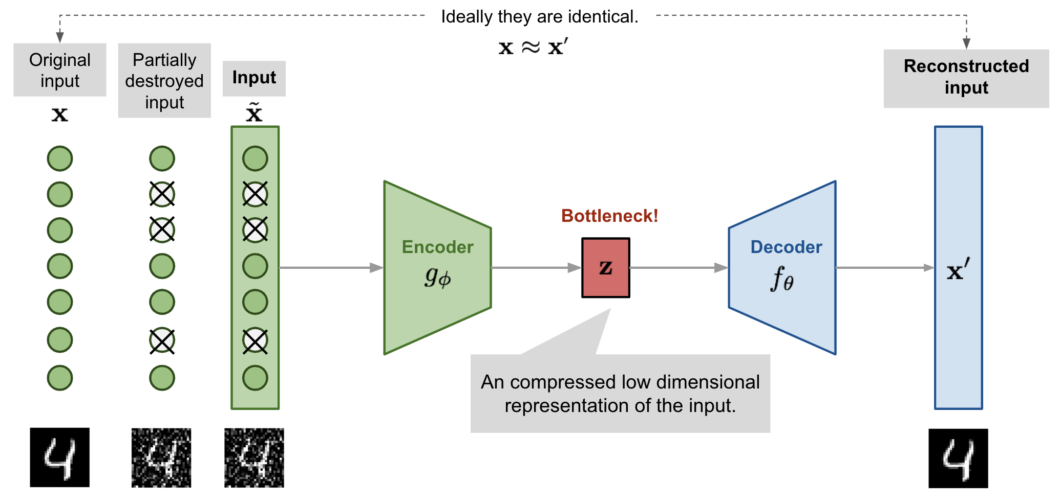

Sparse Autoencoders

A Sparse Autoencoder[3] (SAE) introduces a sparsity constraint on the hidden layer to enforce the model to learn meaningful features of the data. The sparsity constraint ensures that only a small number of neurons are “active” (have high activation values) for any given input, which promotes feature selection and boosts robustness.

Why Sparsity?

The sparsity constraint makes the autoencoder focus on capturing essential features of the data, rather than just memorizing input-output mappings. This is especially useful when:

• The input data has high dimensionality (e.g. images).
• We want to learn interpretable features.
• The dataset is noisy, and only certain features are relevant.

Sparsity is typically enforced by adding a regularization term to the loss function. A common choice is the Kullback-Leibler (KL) divergence, which measures the difference between:

• The average activation of a neuron $ \hat{\rho}_j $, and
• A target sparsity value $ \rho$ (e.g., $\rho = 0.05 $).

$$ \text{Sparsity Penalty} = \sum_{j=1}^m \text{KL}(\rho || \hat{\rho}_j) $$$$ = \sum_{j=1}^m [ \rho \log \frac{\rho}{\hat{\rho}_j} + (1 - \rho) \log \frac{1 - \rho}{1 - \hat{\rho}_j}] $$

where:

• $\hat{\rho}_j$: The average activation of the $j$-th hidden neuron across the dataset.
• $m$: The number of hidden neurons.

$$ L = L_\text{reconstruction} + \beta \cdot \text{Sparsity Penalty}, $$

where $\beta$ is a hyperparameter controlling the importance of sparsity.

K-Sparse Autoencoders

A K-Sparse Autoencoder[4] is a specific type of sparse autoencoder where exactly $k$ neurons in the hidden layer are allowed to be “active” for any given input. This enforces a strict sparsity constraint, where only the top $k$ activations (largest values) are retained, and the rest are set to zero.

How K-Sparsity Works

1. For each input $\mathbf{x} $:
   • Compute the activations of the hidden layer.
   • Retain the top $k $ activations (by magnitude) and set all others to zero.
2. During backpropagation, only the selected $k$ -active neurons contribute to the gradient update.

This approach has the following properties:

• It ensures a fixed level of sparsity ($k $-out-of-$ m $ neurons active).
• It does not require additional sparsity penalties in the loss function, as the sparsity is explicitly enforced.

Variational Autoencoders

One major limitation of standard autoencoders is that their latent space often lacks meaningful structure. When sampling random points from the latent space, the decoder may produce nonsensical or meaningless outputs. This happens because the decoder is not explicitly trained to map random points in the latent space back to realistic data.

For the example before, with VAEs, when sampling random points from the latent space we get a morph of mammals i.e a point between human and jaguar will produce an image of the combined.

To address this issue, the authors of the paper [5] take a different approach. Instead of learning fixed features for a data point, VAEs aim to learn the distribution of the dataset $D$, which we denote as $p_*(\mathbf{x})$.

Explanation

The goal of the VAEs is to generate unseen data by learning a distribution $p_\theta(\mathbf{x})$ that approximates the true distribution $p_*(\mathbf{x})$:

$$ p_\theta(\mathbf{x}) \approx p_*(\mathbf{x}). $$

To achieve this, we maximize the likelihood of the model’s distribution $p_\theta(\mathbf{x})$. Specifically, the objective is to find the parameters $ \theta$ that maximize the likelihood of the observed data:

$$ \theta^* = \arg\max_\theta \prod_{i=1}^n p_\theta(\mathbf{x}^{(i)}). $$$$ \theta^* = \arg\max_\theta \sum_{i=1}^n \log p_\theta(\mathbf{x}^{(i)}). $$$$ p_\theta(\mathbf{x}) = \int_\mathbf{z} p_\theta(\mathbf{x} \vert \mathbf{z}) p_\theta(\mathbf{z}) d\mathbf{z}. $$

The Challenge: Intractability

The problem with directly evaluating this integral is that it is computationally infeasible. Marginalizing over $\mathbf{z}$ requires summing over all possible values of $\mathbf{z}$, which is not practical due to the high dimensionality of the latent space.

The Solution: Variational Approximation

To approximate this integral, VAEs introduce a variational distribution $q_\phi(\mathbf{z} \vert \mathbf{x}) $ as a surrogate for the intractable posterior $ p_\theta(\mathbf{z} \vert \mathbf{x}) $. This approximation enables efficient optimization using the Evidence Lower Bound (ELBO), which we will explore in detail next.

---

REM: Bayes Theorem

$$ P(H|E) = \frac{P(H) \space P(E|H)} {P(E)} $$

where;

$P(H|E)$ - The posterior probability. The probability of getting the hypothesis $H$ given we have observed an event $E$.

$P(H)$ - The prior probability. The probability of getting the hypothesis without the evidence.

$P(E|H)$ - The likelihood/ the update. The probability of observing an event given we have formulated a hypothesis.

$P(E)$ - The marginal likelihood/model evidence. The probability of just observing the event without the hypothesis. Normalizer

---

Variational Inference

$$ p_\theta(\mathbf{z|x}) = \frac{p_\theta(\mathbf{z}) \space p_\theta(\mathbf{x|z})} {p_\theta(\mathbf{x})} $$

We would like to maximize $p_\theta(\mathbf{x})$(which is intractable) but since $p_\theta(\mathbf{x}) = \frac{p_\theta(\mathbf{z,x})}{p_\theta(\mathbf{z|x})}$ getting $p_\theta(\mathbf{z|x})$ would also be computationally expensive as the probability depends on knowledge on $p_\theta(\mathbf{x})$

$$ q_\phi(\mathbf{z|x}) \approx p_\theta(\mathbf{z|x}) $$

where; $q_\phi(\mathbf{z|x})$ is the approximation and $p_\theta(\mathbf{z|x})$ is the target.

Figure2: VAE showing the variational inference

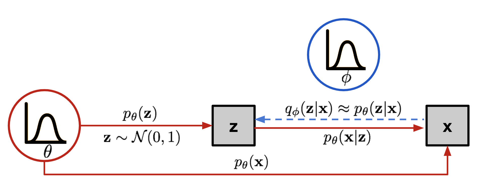
We minimize the gap between the two distributions by using the Kullback-Leibler Divergence

$$ D_\text{KL}( q_\phi(\mathbf{z}\vert\mathbf{x})\space || \space p_\theta(\mathbf{z}\vert\mathbf{x}) ) $$

The above means; the information lost if we adopt the $p_\phi(\mathbf{z|x})$ as our true distribution and $p_\theta(\mathbf{z|x}) $ as the approximation.

$$ \begin{aligned} &\displaystyle D_\text{KL}( q_\phi(\mathbf{z}\vert\mathbf{x}) \| p_\theta(\mathbf{z}\vert\mathbf{x}) ) & \\ &= \int_z q_\phi(\mathbf{z} \vert \mathbf{x}) \log\frac{q_\phi(\mathbf{z} \vert \mathbf{x})}{p_\theta(\mathbf{z} \vert \mathbf{x})} d\mathbf{z} & \\ &= \mathbb{E}_{\mathbf{z}\sim q_\phi(\mathbf{z} \vert \mathbf{x})}[\log \frac{q_\phi(\mathbf{z} \vert \mathbf{x})}{p_\theta(\mathbf{z} \vert \mathbf{x})}] & \\ &=\mathbb{E}_{\mathbf{z}\sim q_\phi(\mathbf{z} \vert \mathbf{x})} [\log q_\phi(\mathbf{z} \vert \mathbf{x}) - \log p_\theta(\mathbf{z} \vert \mathbf{x})] & \\ &=\mathbb{E}_{\mathbf{z}\sim q_\phi(\mathbf{z} \vert \mathbf{x})} \log q_\phi(\mathbf{z} \vert \mathbf{x}) - \mathbb{E}_{\mathbf{z}\sim q_\phi(\mathbf{z} \vert \mathbf{x})}\log p_\theta(\mathbf{z} \vert \mathbf{x}) & \\ &=\mathbb{E}_{\mathbf{z}\sim q_\phi(\mathbf{z} \vert \mathbf{x})} \log q_\phi(\mathbf{z} \vert \mathbf{x}) - \mathbb{E}_{\mathbf{z}\sim q_\phi(\mathbf{z} \vert \mathbf{x})}\log [\frac {p_\theta(\mathbf{z}, \mathbf{x})}{p_\theta(\mathbf{x})}] & \scriptstyle{\text{; Because }p(z \vert x) = p(z, x) / p(x)\text{}} \\ &=\mathbb{E}_{\mathbf{z}\sim q_\phi(\mathbf{z} \vert \mathbf{x})} \log q_\phi(\mathbf{z} \vert \mathbf{x}) - \mathbb{E}_{\mathbf{z}\sim q_\phi(\mathbf{z} \vert \mathbf{x})}\log p_\theta(\mathbf{z} , \mathbf{x}) + \mathbb{E}_{\mathbf{z}\sim q_\phi(\mathbf{z} \vert \mathbf{x})}\log p_\theta(\mathbf{x}) & \\ &=\mathbb{E}_{\mathbf{z}\sim q_\phi(\mathbf{z} \vert \mathbf{x})} \log q_\phi(\mathbf{z} \vert \mathbf{x}) - \mathbb{E}_{\mathbf{z}\sim q_\phi(\mathbf{z} \vert \mathbf{x})}\log p_\theta(\mathbf{z} , \mathbf{x}) + \int{q_\phi(\mathbf{z} \vert \mathbf{x})}\log p_\theta(\mathbf{x}) d\mathbf{z} & \\ &=\mathbb{E}_{\mathbf{z}\sim q_\phi(\mathbf{z} \vert \mathbf{x})} \log q_\phi(\mathbf{z} \vert \mathbf{x}) - \mathbb{E}_{\mathbf{z}\sim q_\phi(\mathbf{z} \vert \mathbf{x})}\log p_\theta(\mathbf{z} , \mathbf{x}) + \log p_\theta(\mathbf{x}) & \scriptstyle {\text{; Because }\int q(z \vert x) dz = 1} \\ &=\mathbb{E}_{\mathbf{z}\sim q_\phi(\mathbf{z} \vert \mathbf{x})} [\log q_\phi(\mathbf{z} \vert \mathbf{x}) - \log p_\theta(\mathbf{z} , \mathbf{x})] + \log p_\theta(\mathbf{x}) & \\ &=\log p_\theta(\mathbf{x}) + \int_z q_\phi(\mathbf{z} \vert \mathbf{x})\log\frac{q_\phi(\mathbf{z} \vert \mathbf{x})}{p_\theta(\mathbf{z}, \mathbf{x})} d\mathbf{z} & \\ &=\log p_\theta(\mathbf{x}) + \int_z q_\phi(\mathbf{z} \vert \mathbf{x})\log\frac{q_\phi(\mathbf{z} \vert \mathbf{x})}{p_\theta(\mathbf{x}\vert\mathbf{z})p_\theta(\mathbf{z})} d\mathbf{z} &\scriptstyle{\text{; Because }p(z, x) = p(x \vert z) p(z)} \\ &=\log p_\theta(\mathbf{x}) + \mathbb{E}_{\mathbf{z}\sim q_\phi(\mathbf{z} \vert \mathbf{x})}[\log \frac{q_\phi(\mathbf{z} \vert \mathbf{x})}{p_\theta(\mathbf{z})} - \log p_\theta(\mathbf{x} \vert \mathbf{z})] & \\ &=\log p_\theta(\mathbf{x}) + D_\text{KL}(q_\phi(\mathbf{z}\vert\mathbf{x}) \| p_\theta(\mathbf{z})) - \mathbb{E}_{\mathbf{z}\sim q_\phi(\mathbf{z}\vert\mathbf{x})}\log p_\theta(\mathbf{x}\vert\mathbf{z}) & \end{aligned} $$

Another way to derive it is using the Jensen’s Inequality

If we rearrange the equation, we should get

$$ \log p_\theta(\mathbf{x}) - D_\text{KL}( q_\phi(\mathbf{z}\vert\mathbf{x}) \| p_\theta(\mathbf{z}\vert\mathbf{x}) ) = \mathbb{E}_{\mathbf{z}\sim q_\phi(\mathbf{z}\vert\mathbf{x})}\log p_\theta(\mathbf{x}\vert\mathbf{z}) - D_\text{KL}(q_\phi(\mathbf{z}\vert\mathbf{x}) \| p_\theta(\mathbf{z})) $$

On the LHS, we have the log likelihood which we would wish to maximize or to say minimize the negative log likelihood. The KL Divergence acts as a regularizer. Since the KL Divergence is always positive, the RHS is the lower bound of the $\log p_\theta(\mathbf{x})$

$$ \text{ELBO} = -\mathbb{E}_{\mathbf{z}\sim q_\phi(\mathbf{z} \vert \mathbf{x})}\log\frac { q_\phi(\mathbf{z} \vert \mathbf{x})}{ p_\theta(\mathbf{z} , \mathbf{x})} $$$$ \text{ELBO} = \mathbb{E}_{\mathbf{z}\sim q_\phi(\mathbf{z} \vert \mathbf{x})}\log\frac { p_\theta(\mathbf{z} , \mathbf{x})}{ q_\phi(\mathbf{z} \vert \mathbf{x})} $$$$ \text{ELBO} = \mathbb{E}_{\mathbf{z}\sim q_\phi(\mathbf{z}\vert\mathbf{x})}\log p_\theta(\mathbf{x}\vert\mathbf{z}) - D_\text{KL}(q_\phi(\mathbf{z}\vert\mathbf{x}) \| p_\theta(\mathbf{z})) $$

The loss function is the negative log likelihood:

$$ \begin{aligned} &L_(\theta, \phi) \\ &=-\log p_\theta(\mathbf{x}) + D_\text{KL}( q_\phi(\mathbf{z}\vert\mathbf{x}) \| p_\theta(\mathbf{z}\vert\mathbf{x}) ) \\ &=-\mathbb{E}_{\mathbf{z} \sim q_\phi(\mathbf{z}\vert\mathbf{x})} \log p_\theta(\mathbf{x}\vert\mathbf{z}) + D_\text{KL}( q_\phi(\mathbf{z}\vert\mathbf{x}) \| p_\theta(\mathbf{z}) ) \\ &\theta^{*}, \phi^{*} = \arg\min_{\theta, \phi} L \end{aligned} $$$$ \nabla_{\theta,\phi} {L} = \nabla_\theta [- \mathbb{E}_{\mathbf{z}\sim q_\phi(\mathbf{z} \vert \mathbf{x})}\log\frac { q_\phi(\mathbf{z} \vert \mathbf{x})}{ p_\theta(\mathbf{z} , \mathbf{x})}] $$

They solved this using the reparameterization trick.

Reparameterization Trick

Lets try backproping from the loss w.r.t $\theta$

$$ L(\theta, \phi) = - \mathbb{E}_{\mathbf{z}\sim q_\phi(\mathbf{z} \vert \mathbf{x})}\log\frac { q_\phi(\mathbf{z} \vert \mathbf{x})}{ p_\theta(\mathbf{z} , \mathbf{x})} $$$$ \begin{aligned} &\nabla_\theta {L} = \nabla_\theta [- \mathbb{E}_{\mathbf{z}\sim q_\phi(\mathbf{z} \vert \mathbf{x})}\log\frac { q_\phi(\mathbf{z} \vert \mathbf{x})}{ p_\theta(\mathbf{z} , \mathbf{x})}] \\ &= \nabla_\theta [\mathbb{E}_{\mathbf{z}\sim q_\phi(\mathbf{z} \vert \mathbf{x})}\log\frac { p_\theta(\mathbf{z} , \mathbf{x})}{ q_\phi(\mathbf{z} \vert \mathbf{x})}] \\ &= \nabla_\theta(\int_z q_\phi(\mathbf{z} \vert \mathbf{x})[\log\ p_\theta(\mathbf{z} , \mathbf{x}) - \log q_\phi(\mathbf{z} \vert \mathbf{x})]d\mathbf{z}) \\ &= \int_z q_\phi(\mathbf{z} \vert \mathbf{x})\nabla_\theta[\log\ p_\theta(\mathbf{z} , \mathbf{x}) - \log q_\phi(\mathbf{z} \vert \mathbf{x})]d\mathbf{z} \\ &= \mathbb{E}_{\mathbf{z}\sim q_\phi(\mathbf{z} \vert \mathbf{x})}\nabla_\theta[\log\ p_\theta(\mathbf{z} , \mathbf{x}) - \log q_\phi(\mathbf{z} \vert \mathbf{x})] \\ &= \mathbb{E}_{\mathbf{z}\sim q_\phi(\mathbf{z} \vert \mathbf{x})}\nabla_\theta[\log\ p_\theta(\mathbf{z} , \mathbf{x}) ] \end{aligned} $$

We can see that the gradient of the expectation is just the expectation of the gradient. We can easily estimate the expectation using Naïve Monte-Carlo sampling.

$$ \nabla_\theta {L} \approx \frac {1}{n} \sum_{i=1} ^n \nabla_\theta[\log\ p_\theta(\mathbf{z} , \mathbf{x}) ] $$

The problem now is the gradient w.r.t $\phi$

$$ \begin{aligned} &\nabla_\phi {L} = \nabla_\phi [- \mathbb{E}_{\mathbf{z}\sim q_\phi(\mathbf{z} \vert \mathbf{x})}\log\frac { q_\phi(\mathbf{z} \vert \mathbf{x})}{ p_\theta(\mathbf{z} , \mathbf{x})}] \\ &= \nabla_\phi (\int_z q_\phi(\mathbf{z} \vert \mathbf{x})[\log\ p_\theta(\mathbf{z} , \mathbf{x}) - q_\phi(\mathbf{z} \vert \mathbf{x})]d\mathbf{z}) \\ &= \int_z \nabla_\phi [q_\phi(\mathbf{z} \vert \mathbf{x}) \cdot\text{ELBO}]d\mathbf{z} \\ &= \int_z q_\phi(\mathbf{z} \vert \mathbf{x}) \cdot \nabla_\phi \text{ELBO} d\mathbf{z} + \int_z \text{ELBO} \cdot \nabla_\phi q_\phi(\mathbf{z} \vert \mathbf{x})d\mathbf{z} \\ &= \mathbb{E}_{\mathbf{z}\sim q_\phi(\mathbf{z} \vert \mathbf{x})} \cdot \nabla_\phi \text{ELBO} + \int_z \text{ELBO} \cdot \nabla_\phi q_\phi(\mathbf{z} \vert \mathbf{x})d\mathbf{z} \end{aligned} $$

You can notice that the first term can be estimated as it is an expectation. However, the second expression is not an expectation and therefore cannot be calculated because we do not have the gradient of $q_\phi$. The solution is to replace $q$ with an equivalent distribution that is not parameterized by $\phi$. This is the reparameterization trick.

$$ \begin{aligned} \mathbf{z} &\sim q_\phi(\mathbf{z}\vert\mathbf{x}^{(i)}) = \mathcal{N}(\mathbf{z}; \boldsymbol{\mu}^{(i)}, \boldsymbol{\sigma}^{2(i)}\boldsymbol{I}) \\ \mathbf{z} &= \boldsymbol{\mu} + \boldsymbol{\sigma} \odot \boldsymbol{\epsilon} \text{, where } \boldsymbol{\epsilon} \sim \mathcal{N}(0, \boldsymbol{I}) \end{aligned} $$

This essentially tranfers the randomness from $\mathbf{z}$ to an external variable $\boldsymbol{\epsilon}$

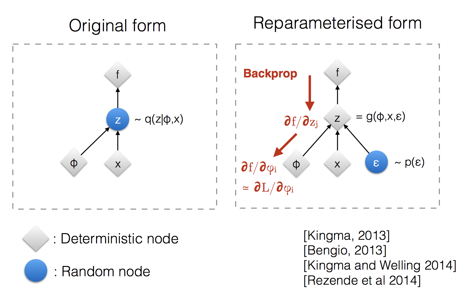
Gradient w.r.t. $ \phi$ with reparameterization.

Using the reparameterization trick, we rewrite $\mathbf{z}$ as:

$$ \mathbf{z} = \boldsymbol{\mu}_\phi(\mathbf{x}) + \boldsymbol{\sigma}_\phi(\mathbf{x}) \odot \boldsymbol{\epsilon}, \quad \boldsymbol{\epsilon} \sim \mathcal{N}(\mathbf{0}, \mathbf{I}). $$$$ \text{ELBO}(\phi, \theta) = \mathbb{E}_{\boldsymbol{\epsilon} \sim \mathcal{N}(\mathbf{0}, \mathbf{I})} \log \frac{p_\theta(\mathbf{z}, \mathbf{x})} {q_\phi(\mathbf{z} \vert \mathbf{x})} $$

The gradient w.r.t. $ \phi$ is:

$$ \nabla_\phi L = - \nabla_\phi \mathbb{E}_{\boldsymbol{\epsilon} \sim \mathcal{N}(\mathbf{0}, \mathbf{I})} \log \frac{p_\theta(\mathbf{z}, \mathbf{x})} {q_\phi(\mathbf{z} \vert \mathbf{x})} $$$$ \nabla_\phi L = - \mathbb{E}_{\boldsymbol{\epsilon} \sim \mathcal{N}(\mathbf{0}, \mathbf{I})} \left[ \nabla_\phi \log p_\theta(\mathbf{z}, \mathbf{x}) - \nabla_\phi \log q_\phi(\mathbf{z} \vert \mathbf{x}) \right]. $$

Breaking Down the Gradients:

1. Gradient of $\log p_\theta(\mathbf{z}, \mathbf{x}) $: Since $\mathbf{z}$ depends on $\phi $ through $\boldsymbol{\mu}_\phi$ and $\boldsymbol{\sigma}_\phi $, the gradient propagates as:

   $$ \nabla_\phi \log p_\theta(\mathbf{z}, \mathbf{x}) = \nabla_\mathbf{z} \log p_\theta(\mathbf{z}, \mathbf{x}) \cdot \nabla_\phi \mathbf{z}. $$

2. Gradient of $\log q_\phi(\mathbf{z} \vert \mathbf{x})$: For a Gaussian distribution $q_\phi(\mathbf{z} \vert \mathbf{x}) = \mathcal{N}(\boldsymbol{\mu}_\phi, \boldsymbol{\sigma}_\phi^2 \mathbf{I})$, the log-probability is:

   $$ \log q_\phi(\mathbf{z} \vert \mathbf{x}) = -\frac{1}{2} \left[ \log (2\pi) + \log (\boldsymbol{\sigma}_\phi^2) + \frac{(\mathbf{z} - \boldsymbol{\mu}_\phi)^2}{\boldsymbol{\sigma}_\phi^2} \right]. $$

   Its gradient w.r.t. $\phi$ is:

   $$ \nabla_\phi \log q_\phi(\mathbf{z} \vert \mathbf{x}) = \nabla_\phi \left( \frac{\mathbf{z} - \boldsymbol{\mu}_\phi}{\boldsymbol{\sigma}_\phi^2} \cdot (\mathbf{z} - \boldsymbol{\mu}_\phi) - \log \boldsymbol{\sigma}_\phi \right). $$

Gradient w.r.t. $\theta$

As derived earlier, the gradient w.r.t. $\theta$ is simpler:

$$ \nabla_\theta L = \mathbb{E}_{\mathbf{z} \sim q_\phi(\mathbf{z} \vert \mathbf{x})} \nabla_\theta \log p_\theta(\mathbf{z}, \mathbf{x}) $$

Using Monte Carlo sampling, this is approximated as:

$$ \nabla_\theta L \approx \frac{1}{n} \sum_{i=1}^n \nabla_\theta \log p_\theta(\mathbf{z}^{(i)}, \mathbf{x}) $$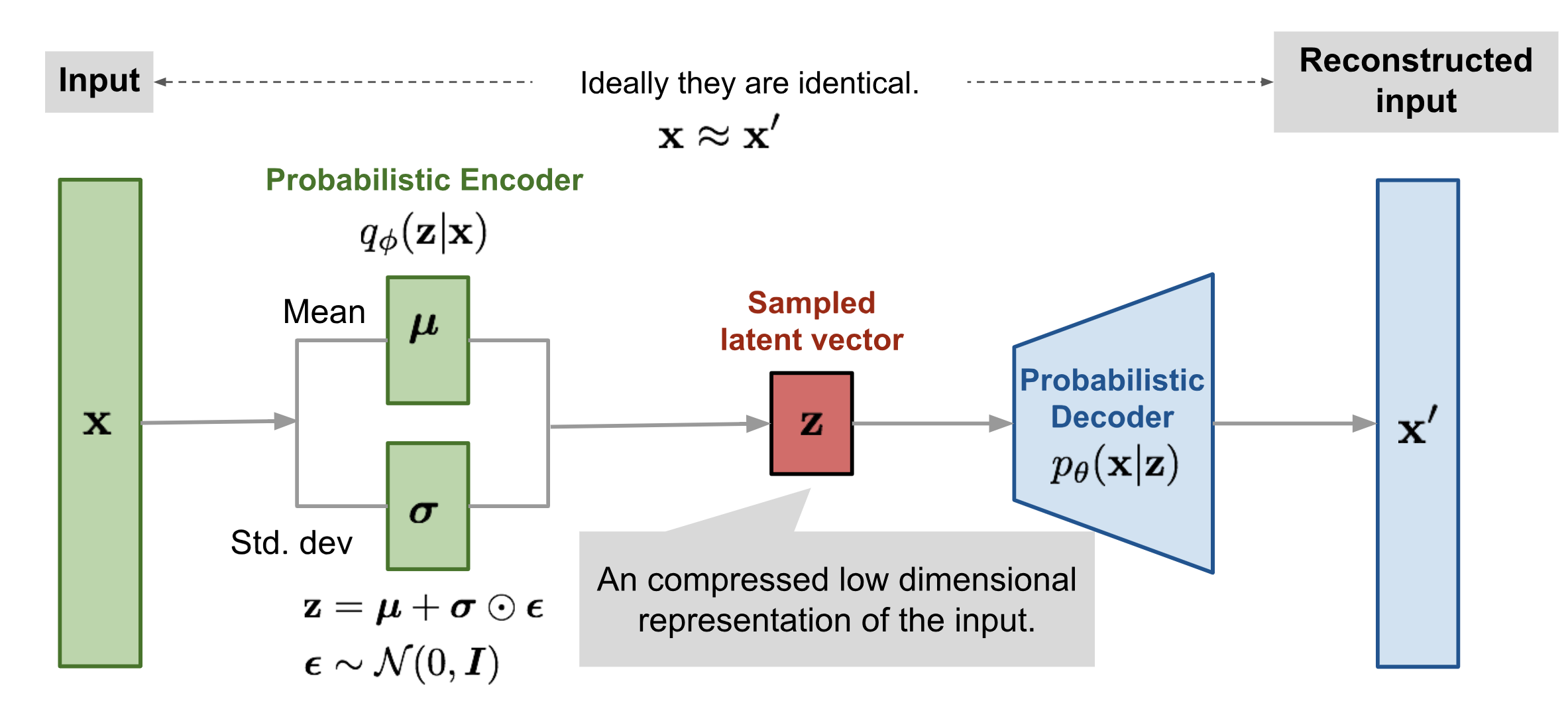

---

References

1. Geoffrey E. Hinton, and Ruslan R. Salakhutdinov. Reducing the dimensionality of data with neural networks (2006).
2. Pascal Vincent, et al. Extracting and composing robust features with denoising autoencoders (2008)
3. Andrew Ng. Sparse Autoencoder
4. Alireza Makhzani, Brendan Frey (2013). k-sparse autoencoder (2014).
5. Diederik P. Kingma, and Max Welling. Auto-encoding variational bayes (2014).