What are optimizers?
Optimizers are mathematical functions or algorithms that aim to reduce the loss value of a model. In simpler terms, optimizers reduce the loss after forward propagation of a model which makes supervised models learn and become ‘smart’.
When training a model, the objective is to minimize the loss/cost function by iteratively updating the model parameters(Weights and Biases) at each epoch.
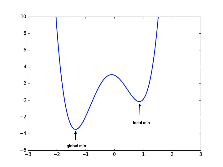
This approach aims in reducing the loss by finding the global minima for the loss function.

To update the parameters or the learning algorithms we use the formula
$$ W_{t+1} = W_{t} - \eta \cdot \nabla L(W_{t}) $$Where:
- $ w_t $: Current weight at time $t$
- $ \eta $: Learning rate
- $ \nabla L(w_t) $: Gradient of the loss function with respect to the weights.
Choosing the right learning rate is crucial because it directly impacts how quickly and effectively a model learns:
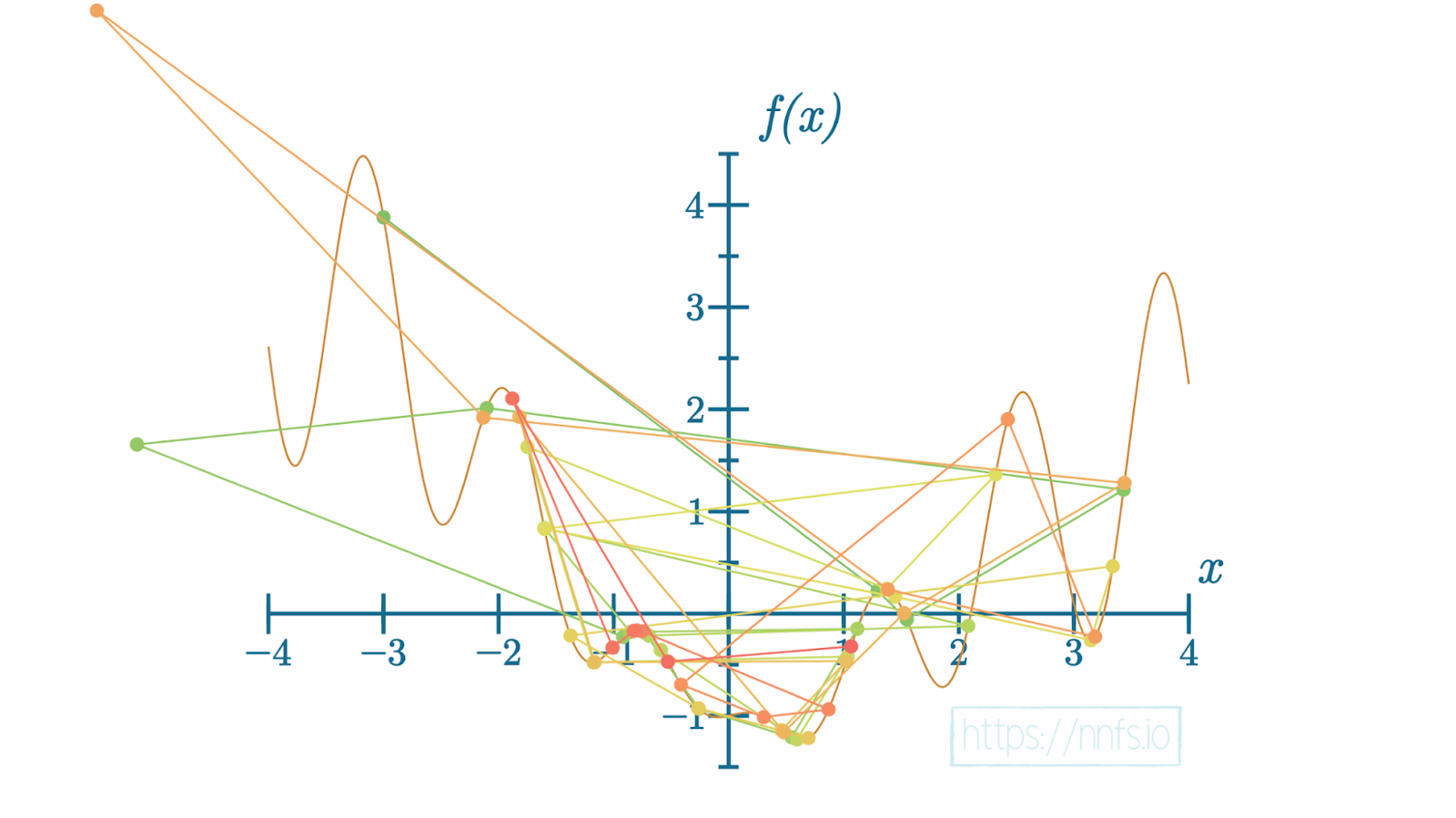
- Too High: If the learning rate is too high, the model might “overshoot” the optimal values, jumping past the minima. It might even cause the training process to diverge, leading to poor performance or failure to converge.

- Too Low: If the learning rate is too low, the model will converge very slowly. Training could take a long time and get stuck in sub-optimal minima because the updates are so tiny that it cannot explore enough of the parameter space to find the global minimum.

The key is finding a balance: the learning rate should be large enough to make noticeable progress but small enough to avoid overshooting and becoming unstable.
In practice, learning rates are often adjusted dynamically using techniques like learning rate schedules or adaptive learning rates, such as those used in optimizers like Adam(adam), to fine-tune the training process.
There are different optimizers in ML and choosing the best optimizers depend on your application i.e. simpler models like a simple feedforward neural network will use a Stochastic Gradient Descent. and bigger models like Transformers using Adam or RMSProp
The optimizers discussed will be gradient-based optimizers for example:
Non-gradient based optimizers like simulated annealing will not be covered.
Stochastic Gradient Descent
The standard SGD involves calculating the gradient one data point at a time and the model’s weights are updated after each data point.
$$ W_{t+1} = W_{t} - \eta \cdot \nabla L(W_{t}) $$where:
- $ \nabla L(W_{t}) $: Gradient of the loss function with respect to weights, computed for a single training sample.
However, the updates can be noisy which leads to high variance in the weight changes and it is also slow to converge.
Batch Gradient Descent
It is the classic form of gradient descent. The gradient is computed using the entire dataset and the weights are updated after processing the entire dataset. This can be very slow if the dataset is very large.
$$ W_{t+1} = W_{t} - \eta \cdot \nabla L(W_{t}) $$where:
- $ \nabla L(W_{t}) $: is now the gradient computed over the entire dataset $X$.
On the bright side it tends to have a smoother convergence.
Mini-batch Gradient Descent
Here, we split the dataset into small slices - batches and calculate the gradient one mini-batch at a time. Updates are also done after processing each mini-batch
$$ W_{t+1} = W_{t} - \eta \cdot \nabla \frac {1}{m} L(W_{t}; x^{(i)}, y^{(i)}) $$Where:
- $ m $: Number of samples in the mini-batch.
- $ x^{(i)}, y^{(i)} $: Input-output pairs in the mini-batch.
- $ \nabla L(W_{t}; x^{(i)}, y^{(i)}) $: Gradient for the 𝑖-th sample in the mini-batch.
This variant of GD is computationally efficient than SGD because it uses vectorized operations over batches and it also helps balance the trade-off between high variance of SGD and the slow convergence of Batch SGD.
Its disadvantage is that it is a bit noisy.
SGD with momentum
The idea of noise has been addresses in gradient descent algorithms where the optimizers take a noisy path to reach the optimal minimum. This noisy approach tends to add computational costs as the number of iterations is increased.
What momentum does is it helps in faster convergence of the loss function by adding the previous update to the current update making it a bit faster.
$$ v_{t+1} = \beta v_{t} + (1 - \beta) \nabla L (W_{t}) $$$$ W_{t+1} = W_{t} - \eta \cdot v_{t+1} $$Without momentum: Imagine a ball on top of a hi;; If you let it just a roll, at any given instant, the motion depends on the steepness of the instant hill. The steeper the hill, the faster the ball goes; the shallower the hill, the slower the ball goes. In other words, the ball moves purely based on the current slope, or gradient, at every point.
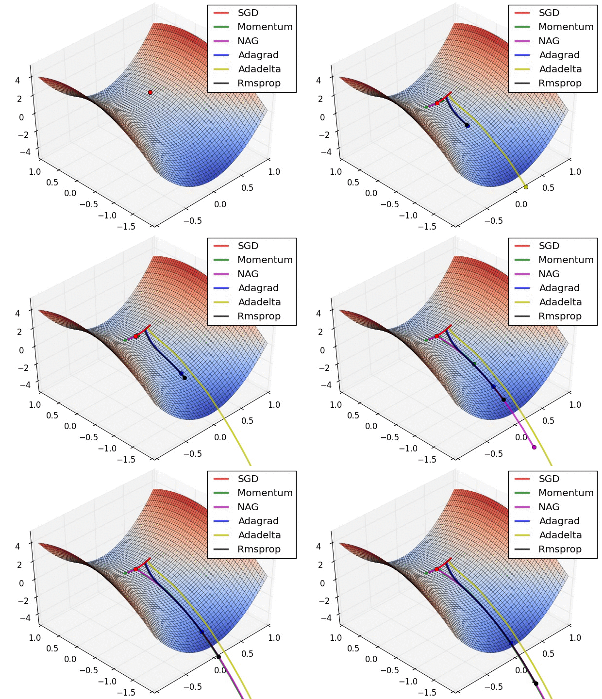
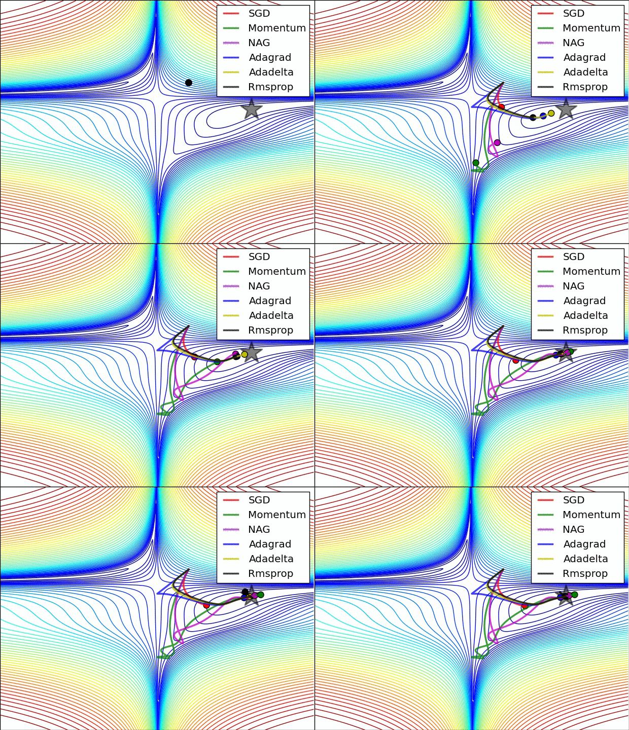
With momentum: Now consider that the ball has some initial velocity, or in other words, momentum, when it starts rolling. The ball, while rolling, does not only respond to the present slope but also caries some of its previous speed. That means even when the slope flattens or reverses its direction, the ball would continue in the same direction for some time due to the built-up momentum. With time, it slows down; the ball would still be moving but would smoothly reach the bottom faster because it would not get stuck in shallow areas. This idea helps to avoid local minima and reduce the number of iterations to converge.
Learning Rate decay
Learning rate decay is a technique where the learning rate starts at a predefined value and gradually decreases over time as the model approaches convergence. This reduction in the learning rate helps to make smaller updates to the model’s parameters, allowing the optimization process to fine-tune the solution more precisely and gradually settle towards the global minimum.
AdaGrad
AdaGrad (Adaptive Gradient Algorithm) is a bit different compared to the others. It is designed to adapt the learning rate of each weight parameter based on its gradient. This helps improve performance for sparse data and leads to faster convergence in some cases.
The key idea behind Adagrad is to adapt the learning rate for each parameter, allowing it to take larger steps for parameters with smaller gradients and smaller steps for parameters with larger gradients. This adjustment happens throughout the training process.
Adagrad keeps track of the sum of squared gradients for each parameter. This means parameters that have been updated frequently will have a larger accumulated gradient, leading to smaller learning rates in the future. The learning rate for each parameter is adjusted based on its historical gradient, so each parameter gets a tailored learning rate.
$$ G_{t, i} = G_{t-1, i} + (\nabla L(w_{t}, i))^2 $$$$ w_{t+1, i} = w_{t, i} - \frac {\eta}{\sqrt{G_{t, i}} + \epsilon} \nabla L(w_{t}, i) $$where:
- $ G_{t, t} $ is the accumulated sum of squared gradients for parameter $ w_i $ at time step $t$
- $\epsilon$ is a small value set to avoid division by zero
Because the learning rate adapts automatically, it reduces the need to finetune the learning rate.
RMSProp
RMSProp (Root Mean Square Propagation) is a variant of AdaGrad designed to solve some Adagrad’s tendecy to reduce the learning rate too aggressively over time.
It introduces a mechanism to “forget” very old gradients by using an exponential moving average over the squared gradients instead of summing them all up like in AdaGrad. This makes it more robust and effective for non-stationary objectives and deep neural networks.
$$ G_{t, i} = \beta G_{t-1, i} + (1- \beta) (\nabla L(w_{t}, i))^2 $$$$ w_{t+1, i} = w_{t, i} - \frac {\eta}{\sqrt{G_{t, i}} + \epsilon} \nabla L(w_{t}, i) $$where:
- $ \beta $ is the decay rate(typically =0.9), controlling how much weight is given to the recent gradients vs past gradients.
If you noticed, RMSProp can be thought of as AdaGrad with momentum (placing more emphasis on recent gradients).
AdaDelta
Like RMSProp, AdaDelta also seeks to address the issue of aggressive decay of the learning rate in AdaGrad. Instead of accumulating all the past squared gradients, AdaDelta limits the accumulation of a window of recent gradients using an exponential moving average similar to RMSProp.
Gradient Accumulation (Exponential Moving Average of Gradients):
$$ E[g^2]_t = \beta E[g^2]_{t-1} + (1 - \beta)(\nabla L(w_t))^2 $$Update Accumulation (Exponential Moving Average of Updates):
$$ E[\Delta w^2]_t = \beta E[\Delta w^2]_{t-1} + (1 - \beta)(\Delta w_t)^2 $$Parameter Update:
$$ \Delta w_t = - \frac{\sqrt{E[\Delta w^2]_{t-1} + \epsilon}}{\sqrt{E[g^2]_t + \epsilon}} \nabla L(w_t) $$Weight Update:
$$ w_{t+1} = w_t + \Delta w_t $$where:
- $ E[g^2]_t $: Exponential moving average of squared gradients at time step $ t $.
- $ E[\Delta w^2]_t $: Moving average of past squared updates.
- $ \beta $: Decay rate (typically $ \beta = 0.9 $).
- $ \sqrt{E[\Delta w^2]_{t-1} + \epsilon} $: Dynamically scaled update size.
However, using AdaDelta is computationally expensive.
Adam
Adam (Adaptive Moment Estimation) is one of the most popular and widely used gradient based algorithms that combined the strengths of both momentum and RMSProp. It leverages on exponentially decaying averages of both past gradients (momentum) and their squared values (adaptive lr).
This means that instead of applying current gradients, we’re going to apply momentums like in the SGD optimizer with momentum, then apply a per-weight adaptive learning rate with the cache as done in RMSProp.
Adam also includes bias correction terms to mitigate the biasness of the gradient and squared gradient towards 0.
Compute Gradients:
Calculate the gradient of the loss function:
Update Biased Estimates:
- First moment (mean of gradients):
- Second moment (variance of gradients):
Bias Correction:
Correct for initial biases in $m_t$ and $v_t$:
Update Parameters:
Use the corrected moments to adjust the weights:
where:
- $\beta_1$: Decay rate for the first moment. Normally set at 0.9.
- $\beta_2$: Decay rate for the second moment (0.999)

