Rolling Your Own GPT

Training a GPT model sounds like a moonshot but it is actually just a series of simple and well-defined steps. At its core, it is just a giant text predictor, fed with tons of data and then allowed to guess the next word. The real challenge is not training it to predict the next word, but to make it produce something useful like answers to your assignment due midnight.😅 You need some special type of training like Reinforcement Learning with Human Feedback (RLHF). Though you can get good responses without RLHF, RLHF is required to make it chatbot-like.

What This Blog Covers

In this blog, we’ll break down the entire pipeline for training a GPT model from scratch. We’ll cover:

1. Pretraining - Teaching GPT to predict the next word using massive datasets.
2. Finetuning - Adapting the model for specific tasks like chatbots or coding assistants.
3. Alignment (RLHF) - Using human feedback to make GPT useful and safe.

By the end, you’ll have a clear roadmap for building your own GPT, whether for research, fun, or world domination. 😈

Introduction

GPT (Generative Pretrained Transformers) models, as the name suggests, are autoregressive generative models based on the Transformer architecture. The reason it is called generative is because the output of the model is new even with the same input.

Before we jump into GPT, let’s briefly recap on the transformer architecture since GPT is essentially a ‘half’ transformer. A full Transformer has both an encoder and a decoder. GPT only uses the decoder.

A transformer[1] is a machine translation neural network that processes input in parallel and uses self-attention to understand the relationship between words/tokens. Unlike older models like RNNs, which process text sequentially, transformers handle entire sequences at once, making them faster and more efficient.

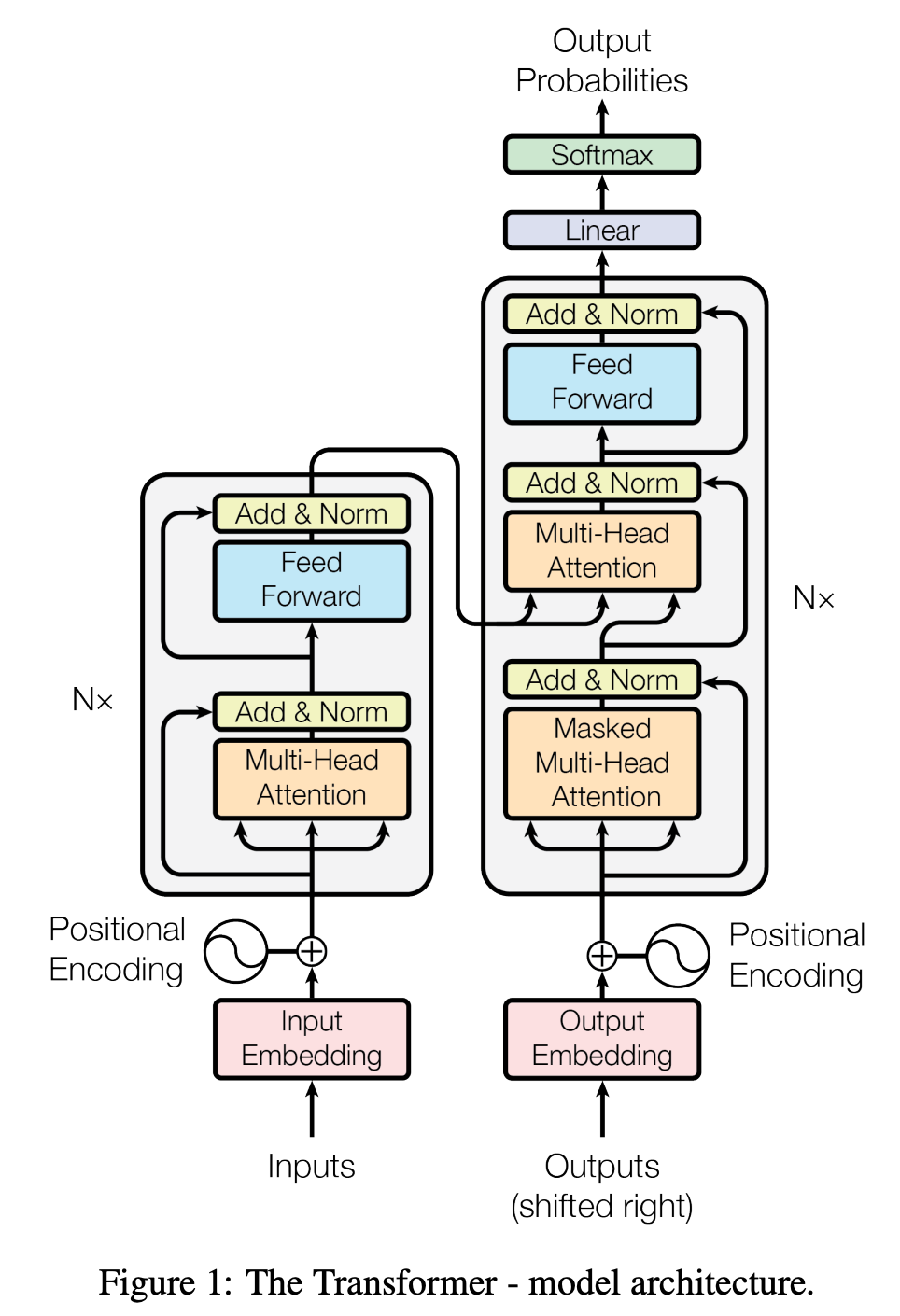
It is composed of two parts:

• Encoder (Left) - Processes the input sequence(used in BERT)
• Decoder (Right) - Generates the output step-by-step(used in GPT)

For more details, please check out Jay Alammar’s [Blog][jay-allamar] or book for in-depth explanation.

GPT models specifically use only the decoder part of the transformer and apply causal masking, meaning each token can only attend to past tokens (not future ones). This makes them great for text generation, but without proper fine-tuning, they might just spit out plausible-sounding nonsense.

Pretraining

Data preparation

After collecting our large text corpus, training data is often filtered and cleaned to remove low-quality content.

Then, the text is converted to numerical format using tokenization. This can be through Byte-Pair Encoding (BPE), SentencePiece or WordPiece which splits words into smaller subword units (tokens). Simpler models can use character level tokens.

Example:

"I love transformers" -> ["I", "love", "trans", "#formers"]

The tokenization process involves a training pipeline that implement encoding - converting a string to a token and decoding - converting a sequence of tokens into a string. Each token is then mapped to a unique ID in a vocabulary which is fed to the model.

Architecture

Each GPT model is built from multiple stacked decoder blocks.

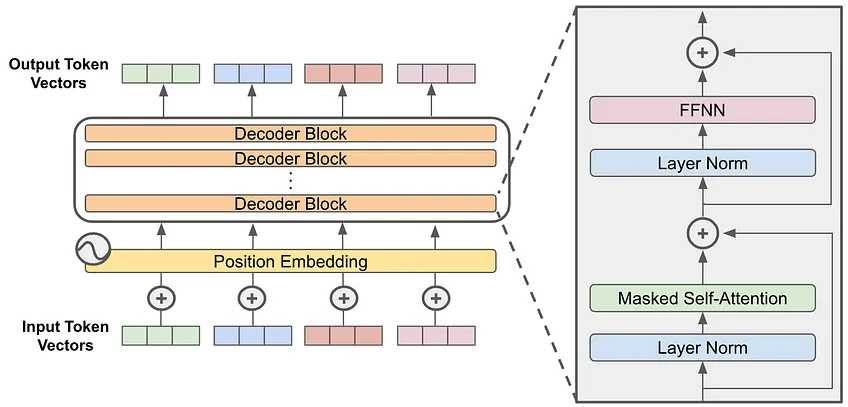
1. Token Embedding - Converts input words/tokens to numerical vectors
2. Positional Encoding - Adds information about word order
3. Decoder Blocks

Token Embedding layer

Once the text has been tokenized into subword units, it needs to be converted into numerical representations that the model can understand.

A token embedding is a learned vector representation of a token. Instead of representing tokens as simple IDs (which don’t capture any meaning), each token is mapped to a high-dimensional vector that contains semantic information.

For example, instead of:

"I" "love" "trans" "#formers" -> [102, 304, 753, 9281]

The embedding layer converts these token IDs into vectors:

[102] -> [0.2, -1.3, 0.7, ..., 1.1]
[304] -> [-0.4, 2.1, -0.9, ..., 0.3]
[753] -> [-0.9, 1.1, 1.2, ..., 0.2]
[9281] -> [1.5, -0.7, 0.8, ..., -1.2]

Each token is now represented as a dense vector of floating-point numbers, typically in a space of 512 to 4096 dimensions, depending on the model size.

It is kind of a look up table with a large matrix $E$ of size (vocab_size x embedding_dim), where each row represents a token and embedding_dim/d_model is the dimension of the vector.

Mathematically, if a token ID is $t_{i}$, the embedding vector is:

where $d$ is the embedding dimension.

Why token embeddings matter:

• Capture Meaning – Similar words have similar embeddings (“dog” and “puppy” will be closer in vector space).
• Reduce Sparsity – Unlike one-hot encoding, embeddings are dense representations, making learning more efficient.
• Enable Transfer Learning – Pretrained embeddings help models generalize better with less data.

Positional Encoding

Since transformers process tokens in parallel, we need positional encoding to retain word order. This is as a result of transformers processing all tokens in parallel and have no built-in understanding of order unlike RNNs.

Instead of relying on recurrence (like RNNs), transformers add a unique positional vector to each token embedding. This encoding is precomputed and added directly to token embeddings before feeding them into the model.

The positional encoding function is defined as:

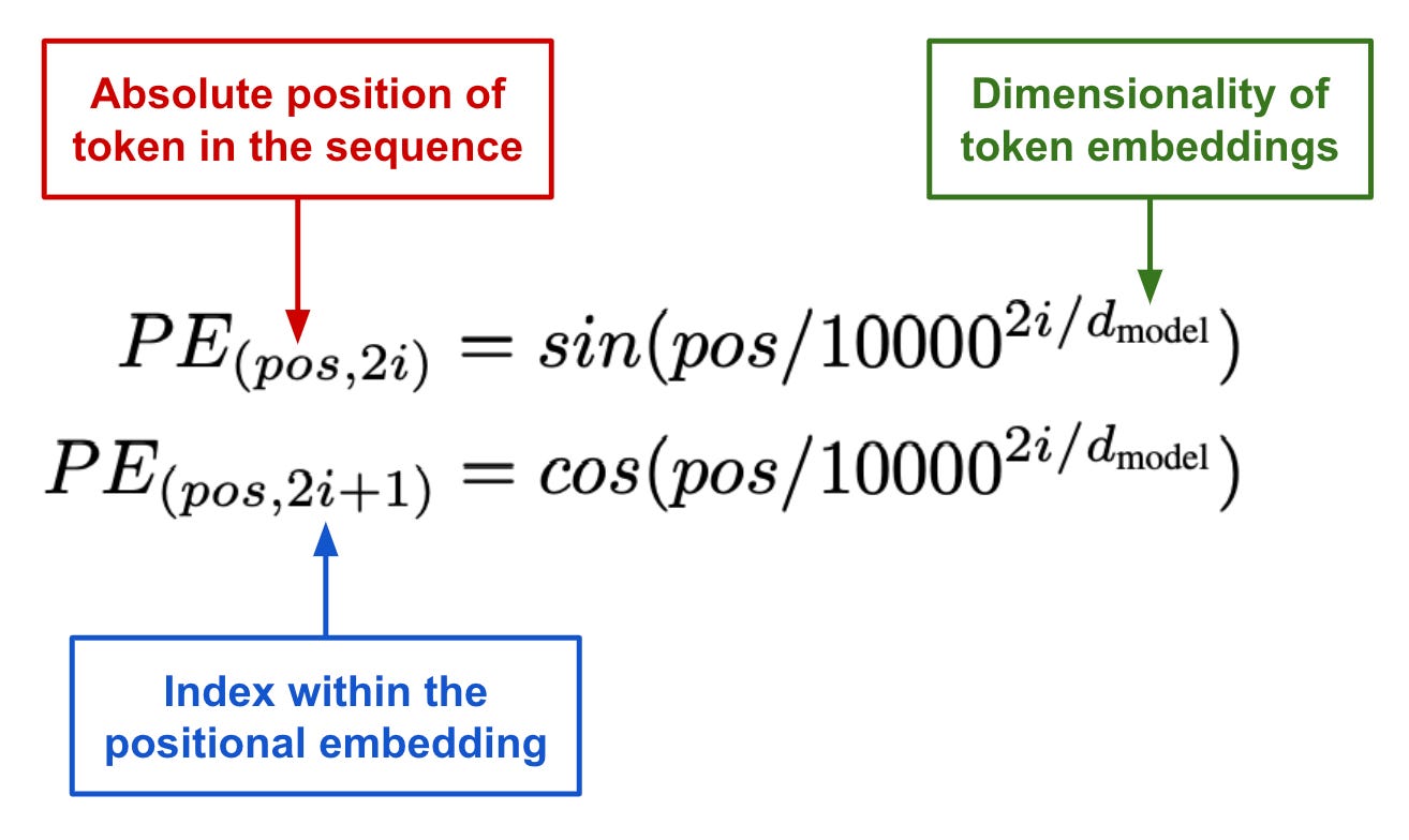
However, most models use learnable positional embeddings instead of sinusoidal encoding while recent architectures like Llama and Mistral use Rotary Positional Embedding which is covered in recent post.

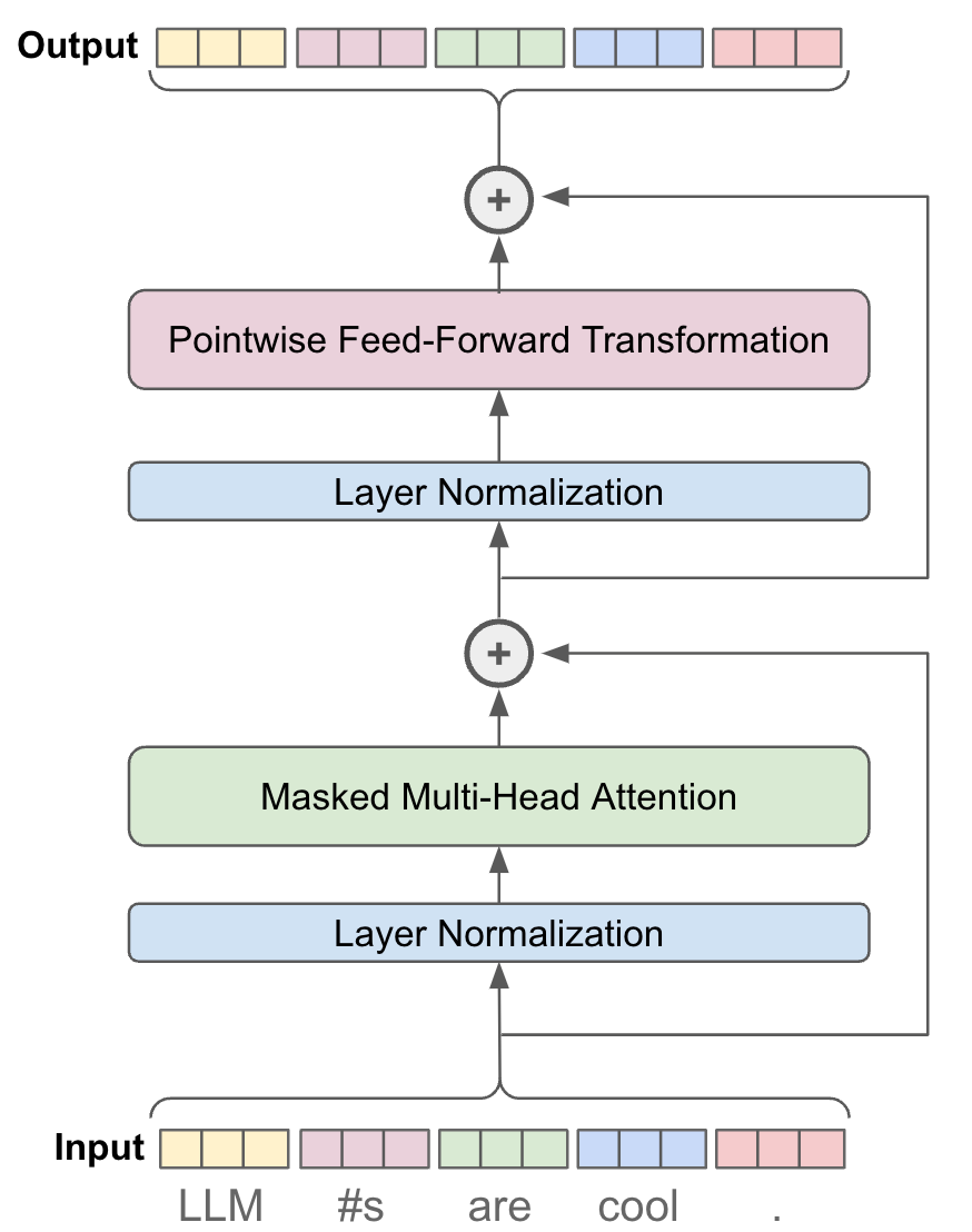
The Decoder Block: The heart of GPT

Each decoder block consists of the following key components:

1. Masked Multi-Head Self-Attention – Ensures each token only attends to past tokens (causal masking).
2. Layer Normalization & Residual Connection – Helps stabilize training.
3. Feedforward Network (FFN) – A fully connected layer that refines token representations.
4. Final Layer Normalization & Residual Connection – Another normalization step to maintain stable gradients.

A typical GPT model stacks multiple decoder blocks (GPT-3.5 has 96 layers).

Masked Multi-Head Self-Attention

Self-attention allows the model to decide which past tokens are most relevant when generating the next token.

Self-Attention Mechanism

Self attention is the core mechanism that enables transformers to understand relationships between words/tokens regardless of their position. Unlike RNNs, which process words sequentially, self-attention allows every word to “pay attention” to other words in the input simultaneously.

Think of it like reading a sentence: when you read a word, your brain doesn’t just process that word in isolation; you subconsciously connect it to previous words, emphasizing some more than others based on context. This is exactly what self-attention does.

Self attention is built around three main concepts:

• Query (Q) - The word asking, “Hey, I am looking for someone who matters? Any Adjective?”
• Key (K) - The rest of the words in the sequence replying, “Am I relevant to you?”
• Value (V) - The actual information being passed along if the relevance is high.

The Q and K also act like a lower dimensional representation of the token’s embeddings.

Now, we measure how much focus each word should have on the others. We do this by computing the dot product between the query of a word and the keys of all other words in the sequence. Higher dot product means the vectors have high similarity and a dot product of zero means the vectors are orthogonal and therefore no similariry.

This results in an attention score matrix where each row represents how much one token should attend to others.

I like to think of it like - Being in a crowd and I am the Query and I am trying to figure out which of these people (Keys) yelling “Hey, It is me!”, might be someone I am looking for. The louder and clearer someones’s voice is to me, the higher the attention score.

To prevent large values from making the softmax overly confident, we scale the scores by the square root of the key dimension $d_{k}$

Next, we normalize the attention scores using the softmax function, turning them into probabilities:

Each word now has a probability distribution showing how much attention it should give to the other words in the sequence.

Each token’s final representation is obtained by multiplying the attention weights with the value vectors.

This means each token gets an updated representation that is a weighted sum of all token values, emphasizing the most relevant words.

Masked Self-Attention

GPT is a causal model, it should never “see the future” when predicting the next word in the sequence. To enforce this, we apply masking of the future tokens when calculating the self-attention.

The mask is a triangular matrix with zeros in the upper right half. Any positions corresponding to future words get $-\inf $ before softmax, making their probabilities effectively zero.

After softmax:

Multi Head Self-Attention

Instead of performing self-attention once, multi-head attention runs multiple attention mechanisms in parallel. Each attention head learns to focus on different aspects of the sentence, capturing various relationships.

Example(The cat sat on the mat):

• One head might focus on subject-verb agreement (“The cat sat”).
• Another head might track prepositional phrases (“sat on the mat”).

Each attention head has it own Q, K and V matrices and produce separate attention outputs which are then concatenated and linearly transformed with another matrix.

Code:

class CausalSelfAttention(nn.Module):
    def __init__(self, d_model: int, n_heads: int, d_k: int, max_seq_length: int):
        super().__init__()

        assert d_model % n_heads == 0

        self.d_model = d_model
        self.n_heads = n_heads
        
        self.d_k = self.d_model // self.n_heads

        self.query_proj = nn.Linear(self.d_model, self.n_heads * self.d_k, bias=False)
        self.key_proj = nn.Linear(self.d_model, self.n_heads * self.d_k, bias=False)
        self.value_proj = nn.Linear(self.d_model, self.n_heads * self.d_k, bias=False)

        self.out_proj = nn.Linear(self.n_heads * self.d_k, self.d_model, bias=False)

        self.register_buffer("mask", torch.tril(torch.ones(max_seq_length, max_seq_length)) * float('-inf'))


    def forward(self, x):
        B, T, C = x.shape

        key = self.key_proj(x).view(B, T, self.n_heads, self.d_k).transpose(1, 2) # B, n_heads, T, d_k
        query = self.query_proj(x).view(B, T, self.n_heads, self.d_k).transpose(1, 2)
        value = self.value_proj(x).view(B, T, self.n_heads, self.d_k).transpose(1, 2)


        attn_weight = (query @ key.transpose(-1, -2)) / math.sqrt(self.d_k)  # B, n_heads, T, T
        attn_weight = attn_weight.masked_fill(self.mask[:T, :T] == 0, float('-inf'))  # apply mask
        attn_weight = F.softmax(attn_weight, dim=-1)  # softmax along the last dimension

        out = (attn_weight @ value).transpose(1, 2).contiguous().view(B, T, C)  # B, T, C

        out = self.out_proj(out)
        return out

Feed Forward Neural Network(FFN)

After the self-attention refines the token representations, the next step is to process these representations independently using a simple neural network.

The FFN allows the model to extract deeper patterns by introducing non-linearity. This lets the model learn complex features. It also refined the token meaning since the token representations are updates in isolation. This ensures more abstract and useful representation.

Recent study[2] also point out that the feedforward network is responsible for storing and retrieval of factual knowledge. The self attention helps identify relevant information from the input and the FFN encode the knowledge by acting as key-value stores. The GELU non-linearlity also enhances memorization.

Example: If the model has learnt that “Paris is the capital of France”, the FFN layers may encode this fact in their weights. When prompted with “The capital of France is…”, it matched with the fact. I would think of this like a simple NN with no convolution learning about the MNIST data.

Code:

class FeedForward(nn.Module):
    def __init__(self, d_model: int):
        super().__init__()

        self.linear1 = nn.Linear(d_model, 4 * d_model)
        self.linear2 = nn.Linear(4 * d_model, d_model)

        self.gelu = nn.GELU(approximate='tanh')

    def forward(self, x):
        return self.linear2(self.gelu(self.linear1(x)))

You might wonder, why expand only to shrink it back? Well, this allows feature extractions and information mixing. The non-linearity also highlights key point i.e higher activations for relevant key points.

Generating Output

At this point, we’ve gone through token embedding, positional encoding, self-attention, and the feedforward network (FFN)—each refining the token representations step by step. Now, it’s time for the final transformation that turns these learned representations into actual words!

Before the model produces output, it applies Layer Normalization (LayerNorm) one last time.

At this stage, each token’s hidden representation has been refined across multiple decoder layers. But the model still operates in vector space, while we need actual word probabilities.

The final linear layer acts as a classifier transforming each token representation into a logit vector which is the size of the vocabulary. Each value in the logit vector represent the likelihood of the token to be the next word in the sequence.

The model need to pick the next word, right? To do so we convert the logits to probabilities using softmax.

This ensures the output probabilities sum to 1, making it a valid probability distribution.

The model selects the token with the highest probability (or samples based on a strategy like temperature or top-k sampling).

Once we have probabilities, the model picks the next token and repeats the process iteratively until:

• A stop token is reached.
• A max length is hit.
• The output meets some quality threshold.

Each new token is fed back into the model, and the process continues autoregressively, token by token until we get a full response.

You can check out the code for pretraining on my github

Finetuning

So far, we have trained a GPT model as a next token predictor. But raw GPT models (Base Models) can still generate nonsense, bias and irrelevant text. To refine them into useful AI assistants, we apply supervised fine-tuning(SFT)

Supervised Fine-Tuning

SFT is the process of training the model on high-quality, task-specific data with labeled examples. Instead of predicting the next token from raw internet text, the model learns from human-curated inputs and outputs to become more aligned with what we want.

For this, we need high quality labelled data on the input and output pairs showing the desired behaviour. This data must be clean, diverse and instruction like.

Example of a dataset:

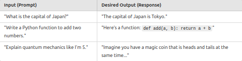
During fine-tuning, the model’s weights are updated using cross-entropy loss between its predictions and the correct answers from the dataset.

Step 1: Model sees an input (e.g. “What is the capital of Japan?”)

Step 2: It generates an output (e.g. “Osaka” ❌)

Step 3: The loss function compares this output to the correct one (“Tokyo” ✅)

Step 4: Backpropagation updates weights to reduce errors.

The fine-tuning objective is still next-token prediction, but now on a curated dataset, ensuring responses become more helpful, accurate, and structured. It is also trained with special tokens <|user|> which marks the beginning of the user’s input and <|assistant|> which marks the beginning of the assistant’s response.

SFT usually takes days to weeks depending on model size and data quantity, but it is far cheaper than training from scratch.

Why SFT is important?

• It improves factual accuracy which in turn reduces hallucinations.
• Makes it user-friendly by ensuring polite, safe, and clear responses.
• Prepares for RLHF

Without SFT, a base GPT model is like a highly intelligent but untrained intern 😅

RLHF

Even after Supervised Fine-Tuning (SFT), the model still has flaws as it can generate biased, misleading, or undesired responses. To further refine its behavior, we apply RLHF, a reinforcement learning approach where human preferences guide the model’s training.

This is because SFT helps the model learn what to say, but RLHF helps it learn how to say it in a way that aligns with human values. Without it, the fine-tuned model may still provide technically correct but unhelpful responses or too verbose or too brief responses.

This is particular in mathematical tasks where we need the model to respond with the steps first then the answer.

Steps in RLHF

1. Supervised finetuning
2. Reward modelling - Training a separate reward model that scores different responses based on human preference
3. Reinforcement Learning with Proximal Policy Optimization (PPO)

Training the reward model

A reward model acts like a quality evaluator for the response.

To train it, we need a dataset where human annotators rank multiple completions of a prompt.

An example dataset:

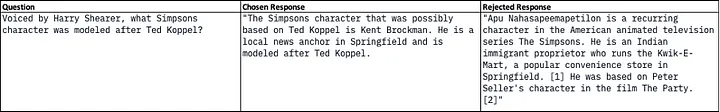
The reward model is then trained to assign higher scores to preferred responses. It learns from human preference data which helps the AI avoid unsafe or misleading outputs. Let’s define a reward function R that assigns a score R(x, y) to a response y given a prompt x.

To train this model, we minimize the loss:

where:

• $y_+$ is the preferred response
• $y_-$ is the less-preferred response
• $\sigma$ is the sigmoid function ($\frac{1}{1 + e^{-z}}$) which ensures the score stay within the valid range.
• $R(x, y_+)$ is the reward assigned to the preferred choice
• $R(x, y_-)$ is the reward assigned to the less-preferred choice

In short, the loss penalizes cases where the preferred option doesn’t get a higher reward than the non-preferred one.

Fine-tuning with Reinforcement Learning

We have a reward model but where does it come in. Well, we use Proximal Policy Optimization (PPO) to train GPT to generate responses that maximize reward scores.

GPT generates a response $y$ for a given input $x$, the reward model $R(x, y)$ assigns a score whether it is a good response of not and finally the PPO adjusts the GPT’s weights to favour responses that get higher scores.

The policy update is:

where:

• $\theta$ are the GPT model weights
• $\alpha$ is the learning rate
• $R(x,y)$ is the reward function.

PPO prevents over-updating by limiting how much the policy can change per step.

References

1. Attention Is All You Need – The original Transformer paper by Vaswani et al. (2017).
2. Jay Alammar’s Blog – An excellent visual explanation of Transformers.
3. Jay Alammar’s Book: Hands-On Large Language Models – A practical guide to understanding and implementing LLMs.
4. “Transformer Feed-Forward Layers Are Key-Value Memories” (Geva et al., 2021)
5. Reinforcement Learning with Human Feedback (RLHF) (Christiano et al., 2017)
6. Language Models Are Few-Shot Learners (Brown et al., 2020) – The GPT-3 paper demonstrating few-shot, zero-shot, and one-shot learning capabilities.
7. Multitask Prompted Training Enables Zero-Shot Task Generalization (Sanh et al., 2022) – A study on how large language models can generalize across tasks.
8. Fine-Tuning Strategies for Large Language Models (Howard & Ruder, 2018) – A paper discussing supervised fine-tuning (SFT) approaches.
9. Byte Pair Encoding (BPE)
10. SentencePiece Tokenizer
11. My GitHub Repository – My personal GPT-2 implementation